Extracting the data ☢️

I’ll download the screenplays for reproducibility purposes. I made a loop in the download.file function for every episode.

episode_name <- c("11_23_45", "2Please-Remain-Calm", "3Open-Wide-O-Earth",
                  "4The-Happiness-Of-All-Mankind", "5Vichnaya-Pamyat")

for(episode in episode_name){
  download.file(
    paste0("https://johnaugust.com/wp-content/uploads/2019/06/Chernobyl_Episode-",
           episode, ".pdf"), 
    paste0(episode, ".pdf"), mode = "wb"
  )
}

Assembling ☢️

The .pdf format is pleasant to work with text. Using the pdf_text function from the pdftools package we can assemble the text into lists. Then we merge all in a tibble.

pdf_names <- paste0(episode_name, ".pdf")
raw_text <- map(pdf_names, pdf_text)

chernobyl <- tibble(episode = pdf_names, text = raw_text) %>% 
  mutate(
    episode =
      case_when(
        .$episode == "11_23_45.pdf"                      ~ "1:23:45",
        .$episode == "2Please-Remain-Calm.pdf"           ~ "Please Remain Calm",
        .$episode == "3Open-Wide-O-Earth.pdf"            ~ "Open Wide, O Earth",
        .$episode == "4The-Happiness-Of-All-Mankind.pdf" ~ "The Happiness Of All Mankind",
        TRUE           ~ "Vichnaya Pamyat"
      )
  )

Tidying ☢️

The tidy format makes easy handling data. Julia Silge and David Robinson defining tidy text format as being a table with one token per row. A token is a meaningful unit of text. With all that said, let’s travel to the north of Ukraine.

chernobyl_tidy <- chernobyl %>% 
  unnest %>% # pdfs_text is a list
  mutate(pag = 1:292) %>% 
  unnest_tokens(word, text, strip_numeric = TRUE) %>%
  mutate(episode = factor(episode,
                          levels = c(
                            "1:23:45", "Please Remain Calm", "Open Wide, O Earth",
                            "The Happiness Of All Mankind", "Vichnaya Pamyat"
                          )))

## Warning: `cols` is now required when using unnest().
## Please use `cols = c(text)`

Filtering

Create a data set without stop words.

chernobyl_tidy_fil <- chernobyl_tidy %>% 
  anti_join(stop_words, by = "word")

characters <- c("legasov", "shcherbina", "dyatlov", "bacho", "pavel",
                "shcherbina", "khomyuk", "toptunov", "akimov", "lyudmilla",
                "bryukhanov", "tarakanov", "fomin", "sitnikov", "gorbachev",
                "vasily", "pikalov", "dmitri", "yuvchenko", "gorbachenko",
                "stolyarchuk", "boris", "charkov", "vetrova", "shadov",
                "garo", "stepashin")

Ploting Frequency ☢️

reorder_within <- function(x, by, within, fun = mean, sep = "___", ...) {
  new_x <- paste(x, within, sep = sep)
  stats::reorder(new_x, by, FUN = fun)
}
scale_x_reordered <- function(..., sep = "___") {
  reg <- paste0(sep, ".+$")
  ggplot2::scale_x_discrete(labels = function(x) gsub(reg, "", x), ...)
}
chernobyl_tidy_fil %>% 
  group_by(episode, word) %>% 
  count(sort = TRUE) %>% 
  filter(!word %in% characters) %>% 
  group_by(episode) %>% 
  top_n(10, n) %>%
  ungroup() %>%
  ggplot(aes(reorder_within(word, n, episode), n))+
  geom_col(fill = "#0D0D0D")+
  scale_x_reordered()+
  facet_wrap(~episode, scales = "free_y")+
  coord_flip()+
  theme_minimal()+theme(legend.position = "none")+
  labs(caption = "Viz: @RiversArthur \nData: https://johnaugust.com ",
       x = NULL, y = NULL, title = "Most frequent words",
       subtitle = "Without stop words and characters names")+
  theme(panel.background = element_rect(fill = "#F2E205"), strip.text = element_text(size = 13),
        panel.grid.major.y = element_blank(), panel.grid.major = element_blank(),
        axis.text.y = element_text(size = 10),
        plot.background = element_rect(fill = "#F2E205", color = "#F2E205"))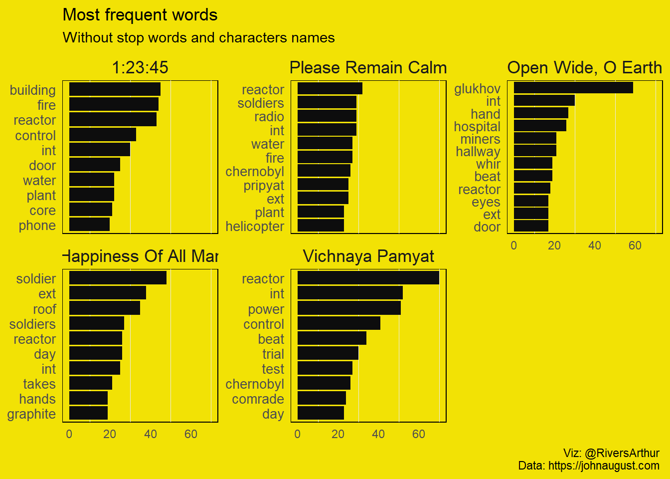

Here we see the most words in each episode. I’ve filtered the stop words and character names because Legasov appears just too much in every episode besides the first one. After that it was hole some see the major topics appears. Remember the spoiler embargo for this miniseries isn’t over yet. So, we can say that the first episode is all about a building or reactor that may or may not be on fire. The second also has fire but has water too and soldiers uses radio. Well you got the idea. Next, we’ll see what the different episodes have of different among them.

TF-IDF or Я люблю тебя родина ☢️

The idea of tf-idf is to find the important words for the content of each episode by decreasing the weight for the commonly used words and increasing the weight for words that are not used very much.

chernobyl_tidy_fil_per_epi <- chernobyl_tidy_fil %>% 
  count(episode, word, sort = TRUE) %>% 
  ungroup()

total_words <- chernobyl_tidy_fil_per_epi %>% 
  group_by(episode) %>% 
  summarise(total = sum(n))

chernobyl_tidy_fil_per_epi <- left_join(chernobyl_tidy_fil_per_epi, total_words,
                                        by = "episode")

chernobyl_tidy_fil_per_epi <- chernobyl_tidy_fil_per_epi %>%
  bind_tf_idf(word, episode, n )

chernobyl_tidy_fil_per_epi %>%
  arrange(desc(tf_idf)) %>%
  mutate(word = factor(word, levels = rev(unique(word)))) %>%
  group_by(episode) %>%
  top_n(10) %>% 
  ungroup %>% 
  ggplot(aes(reorder_within(word, tf_idf, episode), tf_idf)) +
  geom_col(show.legend = FALSE, fill = "#0D0D0D")+
  facet_wrap(~episode, ncol = 1, scales = "free_y") + 
  coord_flip()+
  scale_x_reordered()+ scale_y_continuous(labels = c("Lower TF-IDF",
                                                     "Higher TF-IDF"),
                                          breaks = c(0.001,.033))+
  theme_minimal()+theme(legend.position = "none")+
  labs(caption = "Viz: @RiversArthur \nData: https://johnaugust.com ",
       x = NULL, y = NULL, title = "Highest tf-idf words in each of Chernobyl's episodes",
       subtitle = "Top 10 Words")+
  theme(panel.background = element_rect(fill = "#F2E205"), strip.text = element_text(size = 13),
        panel.grid.major = element_blank(), panel.grid = element_blank(),
        axis.text.y = element_text(size = 12),
        plot.background = element_rect(fill = "#F2E205", color = "#F2E205"))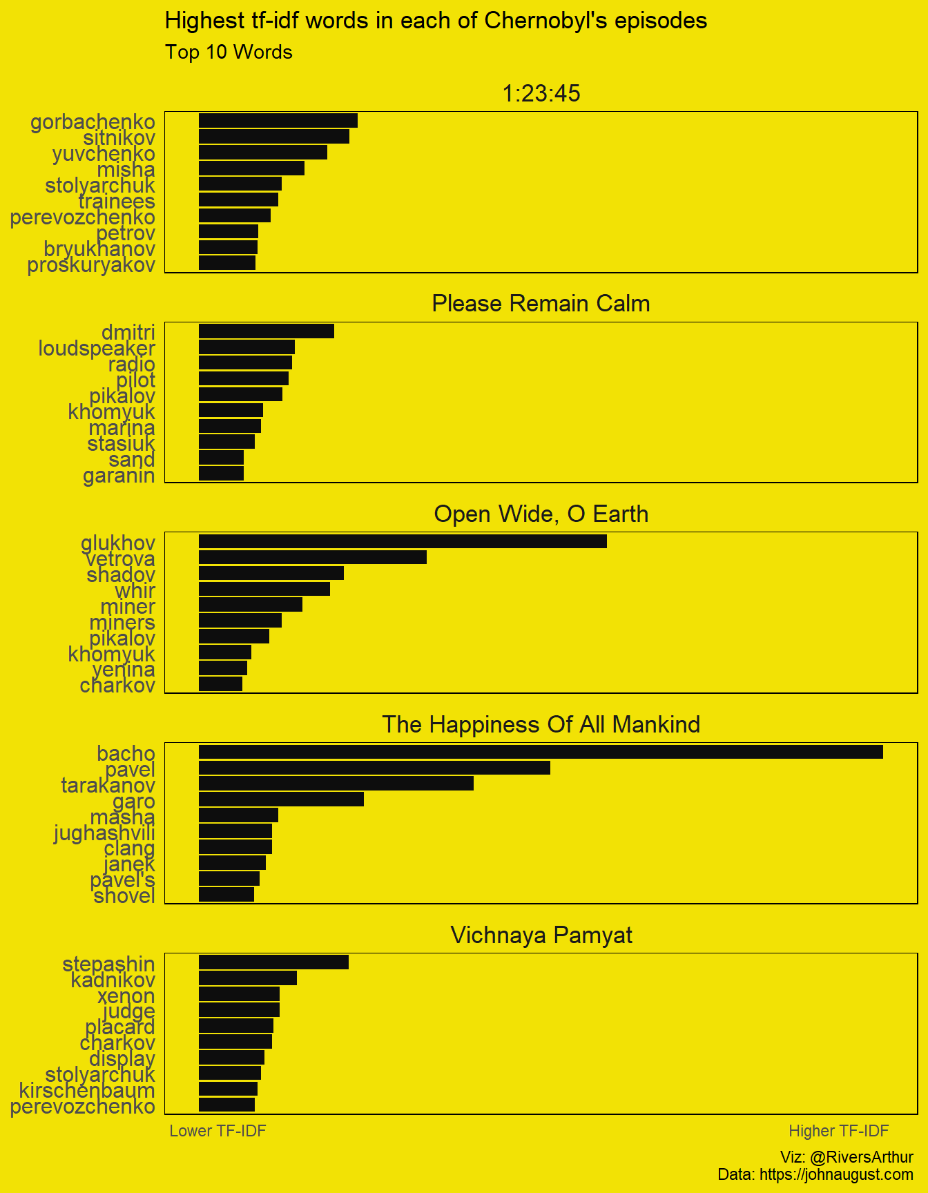

This time we don’t filter the most frequent words because their weight is important to see the most important words in each episode. Aside for the diverse Russian character names (that may indicate several new characters per episode), there’s also some key words. The immediate aftermath of the catastrophe in the second episode is marked by loudspeaker. The badass miners that that enter headfirst in solving the problem on the third episode also arise in the top 10.

chernobyl_bigram <- chernobyl_tidy_fil %>% 
  unnest_tokens(bigram, word, token = "ngrams", n = 2) %>%
  separate(bigram, c("word1", "word2"), sep = " ") %>%
  filter(!word1 %in% stop_words$word,
         !word2 %in% stop_words$word) %>%
  group_by(episode) %>%
  count(word1, word2, sort = TRUE) %>%
  filter(n > 4) %>% 
  graph_from_data_frame()

a <- grid::arrow(type = "closed", length = unit(.10, "inches"))

ggraph(chernobyl_bigram, layout = "fr") +  
  geom_edge_link(aes(edge_alpha = n), show.legend = FALSE, arrow = a, end_cap = circle(.05, 'inches')) +
  geom_node_point(color = "#0D0D0D", size = 4, alpha = 0.5) +  
  geom_node_text(aes(label = name), vjust = 1, hjust = 1, color = "#0D0D0D", size = 4) +  
  theme_void()+
  labs(caption = "Viz: @RiversArthur \nData: https://johnaugust.com ")+
  theme(panel.background = element_rect(fill = "#F2E205"),plot.background = element_rect(fill = "#F2E205",
                                                                                         color = "#F2E205"))

Sentiment ☢️

Now let’s perform a sentiment analysis on the bigram data, we can examine how often sentiment-associated words are preceded by not or other negative words. We could use this to ignore or even reverse their contribution to the sentiment score.

afinn <- get_sentiments(lexicon = "afinn")
negation_words <- c("not", "no", "never", "without")

negative_words <- chernobyl_tidy %>% 
  unnest_tokens(bigram, word, token = "ngrams", n = 2) %>%
  separate(bigram, c("word1", "word2"), sep = " ") %>%
  filter(word1 %in% negation_words) %>% 
  inner_join(afinn, by = c("word2" = "word")) %>% 
  count(word2, value, sort = TRUE) %>% 
  ungroup()

negative_words %>% 
  mutate(contribution = value * n) %>% 
  arrange(desc(abs(contribution))) %>% 
  head(20) %>% 
  mutate(word2 = fct_reorder(word2, contribution)) %>% 
  ggplot(aes(word2, n * value, fill = n * value > 0))+
  geom_col(show.legend = FALSE)+
  scale_fill_manual(values = c("#9CFF59", "white"))+
  labs(x = "Words preceded by negative words", 
       title = "Words that may deceive the analises",
       y = "Sentiment score * number of occurrences",
       caption = "Viz: @RiversArthur \nData: https://johnaugust.com ")+
  coord_flip()+
  theme(panel.background = element_rect(fill = "#F2E205"),panel.grid.major.y = element_blank(),
        panel.grid.major = element_blank(),
        plot.background = element_rect(fill = "#F2E205",
                                       color = "#F2E205"))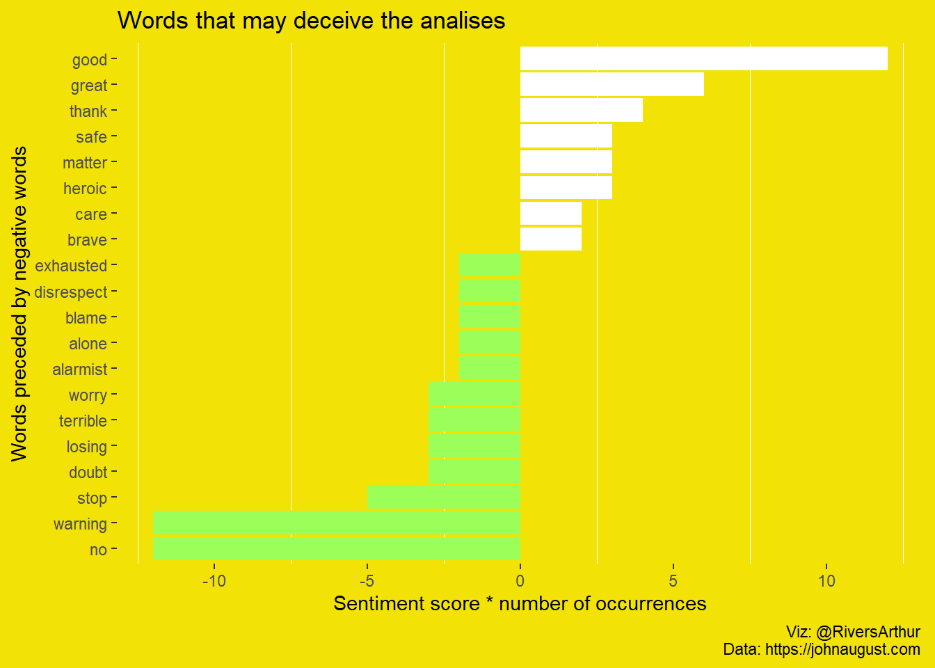

#chernobyl_tidy %>% 
#  inner_join(afinn %>% 
#               filter(value < 0)) %>% 
#  count(word, sort = TRUE)

cher_afin <- chernobyl_tidy %>% 
  inner_join(get_sentiments("afinn")) %>%
  group_by(index = pag %/% 5) %>% 
  summarise(sentiment = sum(value)) %>% 
  mutate(method = "AFINN")

cher_bing_ncr <- bind_rows(
  chernobyl_tidy %>% 
    inner_join(get_sentiments("bing")) %>% 
    mutate(method = "BING"),
  chernobyl_tidy %>% 
    inner_join(get_sentiments("nrc") %>% 
                 filter(sentiment %in% c("positive", "negative"))) %>% 
    mutate(method = "NCR")
) %>%  
  count(method, index = pag %/% 5, sentiment) %>% 
  spread(sentiment, n, fill = 0) %>% 
  mutate(sentiment = positive - negative)

bind_rows(
  cher_afin, cher_bing_ncr) %>% 
  ggplot(aes(index, sentiment, fill = method)) +
  geom_col(show.legend = FALSE)+
  geom_vline(xintercept = c(12*1:4))+
  facet_wrap(~method, ncol = 1, scales = "free_y")+
  scale_fill_manual(values = c("AFINN" = "#9CFF59", "BING" = "#000000",
                               "NCR" = "#F2E205"))+
  labs(caption = "Viz: @RiversArthur \nData: https://johnaugust.com ",
       subtitle = "Each box is one episode",
       x = NULL, y = "Sentiment score", title = "Diferent sentiments scores by different methods")+
  theme_minimal()+
  theme(panel.background = element_rect(fill = "white"), strip.text = element_text(size = 13),
        panel.grid.major = element_blank(),
        axis.text.y = element_text(size = 10),
        plot.background = element_rect(fill = "white", color = "white"))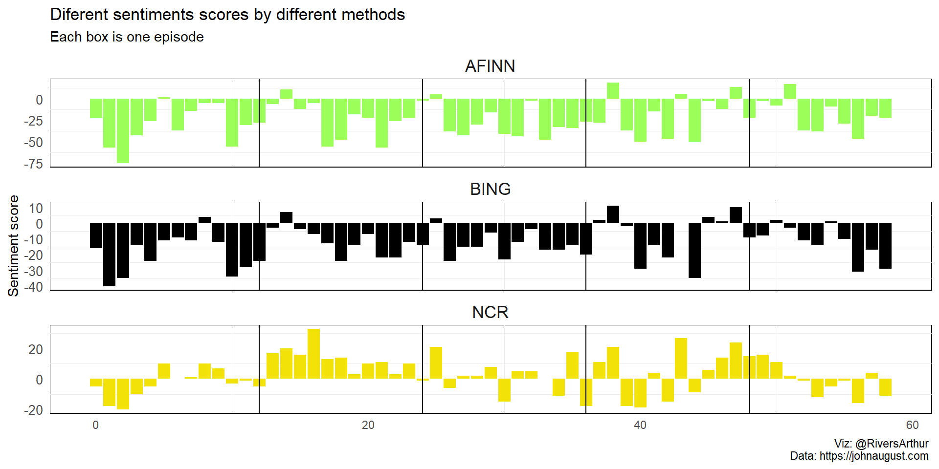

And there you go, isn’t the happiest series in the word but it sure was captivating.

Now we wait the Russian response.